Thouless pumps and winding invariant
Hamiltonians with parameters
Previously, when studying the topology of systems supporting Majoranas (both the Kitaev chain and the nanowire), we were able to calculate topological properties by studying the bulk Hamiltonian \(H(k)\).
There are two points of view on this Hamiltonian. We could either consider it a Hamiltonian of an infinite system with momentum conservation
or we could equivalently study a finite system with only a small number of degrees of freedom (corresponding to a single unit cell), and a Hamiltonian which depends on some continuous periodic parameter \(k\).
Of course, without specifying that \(k\) is the real space momentum, there is no meaning in bulk-edge correspondence (since the edge is an edge in real space), but the topological properties are still well-defined.
Sometimes we want to know how a physical system changes if we slowly vary some parameters of the system, for example a bias voltage or a magnetic field. Because the parameters change with time, the Hamiltonian becomes time-dependent, namely
The slow adiabatic change of parameters ensures that if the system was initially in the ground state, it will stay in the ground state, so that the topological properties are useful.
A further requirement for topology to be useful is the periodicity of time evolution:
The period can even go to \(\infty\), in which case \(H(-\infty) = H(+\infty)\). The reasons for the requirement of periodicity are somewhat abstract. If the Hamiltonian has parameters, we’re studying the topology of a mapping from the space of parameter values to the space of all possible gapped Hamiltonians. This mapping has nontrivial topological properties only if the space of parameter values is compact.
For us, this simply means that the Hamiltonian has to be periodic in time.
Of course, if we want systems with bulk-edge correspondence, then in addition to \(t\) our Hamiltonian must still depend on the real space coordinate, or the momentum \(k\).
Quantum pumps
In the image below (source: Chambers’s Encyclopedia, 1875, via Wikipedia) you see a very simple periodic time-dependent system, an Archimedes screw pump.

The changes to the system are clearly periodic, and the pump works the same no matter how slowly we use it (that is, change the parameters), so it is an adiabatic tool.
What about a quantum analog of this pump?
Let’s take a one-dimensional region, coupled to two electrodes on both sides, and apply a strong sine-shaped confining potential in this region. As we move the confining potential, we drag the electrons captured in it.
So our system now looks like this:
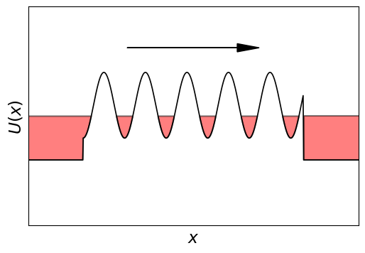
It is described by the Hamiltonian
As we discussed, if we change \(t\) very slowly, the solution will not depend on how fast \(t\) varies.
When \(A \gg 1 /m \lambda^2\) the confining potential is strong, and additionally if the chemical potential \(\mu \ll A\), the states bound in the separate minima of the potential have very small overlap.
The potential near the bottom of each minimum is approximately quadratic, so the Hamiltonian is that of a simple Harmonic oscillator. This gives us discrete levels of the electrons with energies \(E_n = (n + \tfrac{1}{2})\omega_c\), with \(\omega_c = \sqrt{A/m\lambda^2}\) the oscillator frequency. In the large A limit, the states in the different minima are completely isolated so that the energy bands are flat with vanishing (group) velocity \(d E_n(k)/d k=0\) of propagation.
We can numerically check how continuous bands in the wire become discrete evenly spaced bands as we increase \(A\):
So unless \(\mu = E_n\) for some \(n\), each minimum of the potential contains an integer number of electrons \(N\).There are a large number of states at this energy and almost no states at \(\mu\) away from \(E_n\).
Since electrons do not move between neighboring potential minima, so when we change the potential by one time period, we move exactly \(N\) electrons.
Why are some levels in the band structure flat while some are not?
Quantization of pumped charge
As we already learned, integers are important, and they could indicate that something topological is happening.
At this point we should ask ourselves these questions: Is the discreteness of the number of electrons \(N\) pumped per cycle limited to the deep potential limit, or is the discreteness a more general consequence of topology?
Thought experiment
Let us consider the reservoirs to be closed finite (but large) boxes. When the potential in the wire is shifted the electrons clearly move from the left to the right reservoir. How do the reservoirs accomodate these electrons?
Since the Hamiltonian is periodic in time, the Hamiltonian together with all its eigenstates return to the initial values at the end of the period. The adiabatic theorem guarantees that when the Hamiltonian changes slowly the eigenstates evolve to an eigenstate that is adjacent in energy.

We indeed see that the levels move up and down in energies. The states that don’t shift in energy are the ones trapped in the minima of the periodic potential.
To understand better what is happening, let us color each state according to the position of its center of mass, with red corresponding to the left reservoir, blue to the right one, and white to the middle of the system.

We see that the states in the gaps between the wire bands belong to either of the two reservoirs. States in the left reservoir turn out to move down in energy and ones in the right reservoir move up in energy (right now this is numerical—we will see why later).
Let us imagine we park our Fermi energy (i.e. the energy that separates completely occupied and completely empty states) in the gap where there are few states.
With time, an empty level in the left reservoir moves from above the Fermi level to a state below the Fermi level. The occupation of this state cannot change in this process because of the adiabatic theorem. Therefore after the pumping cycle is over the left reservoir has an empty state below the Fermi level i.e. one less electron. The reverse process happens in the right lead so that it has one extra electron.
So the electron that was transferred in the wire from the left reservoir to the right came from emptying the highest energy occupied state one the left and occupying the lowest energy unoccupied state on the right.
More generally, while levels do not have to move as shown in the figure, the energy level structure of the periodic in time Hamiltonian has to return to itself. The number (possibly negative) of levels in the left reservoir that crossed from being above the Fermi level to below must exactly be the change in charge of the left reservoir. This is an INTEGER.
Therefore, our thoughts about “where the electrons came from” leads us to an interesting conclusion: The number of charges pumped in an adiabatic pumping cycle (independent of the strength \(A\)) is an integer (possibly \(0\)).
Furthermore, it is an integer as long as the wire is gapped at the chosen Fermi level (so as to isolate the reservoirs).
So without doing any calculations, we can conclude that:
The number of electrons pumped per cycle of a quantum pump is an integer as long as the bulk of the pump is gapped. Therefore it is a topological invariant.
Counting electrons through reflection.
The expression for the pumped charge in terms of the bulk Hamiltonian \(H(k, t)\) is complicated.
It’s an integral over both \(k\) and \(t\), called a Chern number or in other sources a TKNN integer. Its complexity is beyond the scope of our course, but is extremely important, so we will have to study it… next week.
There is a much simpler way to calculate the same quantity using scattering formalism. This follows from returning to understanding how energy levels in the reservoir move as a function of time.
Consider levels in the energy gap of the wire so that the levels near the Fermi energy are confined to the reservoir. Now all the levels in the reservoir are quantized, and are standing waves, so they are equal weight superpositions of waves going to the left \(\psi_L\) and to the right \(\psi_R\),
where the wave number \(k_n\) is of course a function of energy. The relative phase shift \(\phi\) is necessary to satisfy the boundary condition at \(x=0\), where \(\psi_L = r \psi_R\), and so \(\exp(i \phi) = r\). The energies of the levels are determined by requiring that the phases of \(\psi_L\) and \(\psi_R\) also match at \(x = -L\). These boundary conditions lead to the relation
Changing the phase continuously in time \(t\) by \(2\pi\) evolves \(k_n\) from \((2 L)^{-1}[2n\pi+\phi]\) to \((2L)^{-1}[2n\pi+2\pi+\phi]=2k_{n+1}L\). This means that the change in phase \(\phi\) results in the state with index \(n\) evolving into an index \(n+1\). Thus, the winding of phase \(\phi\) by \(2\pi\) also changes the wave-function \(\psi_n \rightarrow \psi_{n+1}\).
As discussed in the previous paragraph, such a movement of energy level in the reservoir is associated with transfer of charge between the reservoir through the wire.
We conclude that if the reflection phase \(\phi\) from the wire advances by \(2\pi\), this corresponds to a unit charge pumped across the wire.
It’s very easy to generalize our argument to many modes. For that we just need to sum all of the reflection phase shifts, which means we need to look at the phase of \(\det r\).
We conclude that there’s a very compact relation between charge \(dq\) pumped by an infinitesimal change of an external parameter and the change in reflection matrix \(dr\):
While we derived this relation only for the case when all incoming particles reflect, and \(r\) is unitary, written in form of trace it also has physical implications even if there is transmission.¹
Let’s check if this expression holds to our expectations. If \(||r||=1\), this is just the number of times the phase of \(\det r\) winds around zero, and it is certainly an integer, as we expected.
This provides an independent argument (in addition to the movement of energy levels from the last section ) for why the pumped charge is quantized as long as the gap is preserved.
Applying the topological invariant
We know now how to calculate the pumped charge during one cycle, so let’s just see how it works in practice.
The scattering problem in 1D can be solved quickly, so let’s calculate the pumped charge as a function of time for different values of the chemical potential in the pump.

In the left plot, we show the band structure, where the different colors correspond to different chemical potentials. The right plot shows the corresponding pumped charge. During the pumping cycle the charge may change, and the relation between the offset \(\phi\) of the potential isn’t always linear. However we see that after a full cycle, the pumped charge exactly matches the number of filled levels in a single potential well.